Natural Frequency and Damping of a Second Order System and Issues with Aliasing

Let's estimate a second order system

Parts List

1. Laptop

2. CPX + USB Cable

3. This project will require you to build something or utilize something that varies. I’ll explain a bit more on that later but because this lab is variable the parts list will be different depending on what you do. The minimum parts list is shown below.

A second order system undergoing free motion will have dynamics that look like this

$$\ddot{\theta}+2\zeta w_n \dot{\theta}+w_n^2=0$$

In this case, the solution to the above equation can be solved using standard second order differential equation techniques to obtain the solution below.

$$\theta(t) = \theta_0e^{-\sigma t}cos(\omega_dt)$$

$$w_n = \sqrt{\sigma^2 +\omega_d^2}$$

$$\zeta = \frac{\sigma}{\omega_n}$$

Looking at the equations you can see that if you the time series of the oscillations are known, the damping constant and damped natural frequency can be obtained. These two values can be combined to obtain the natural frequency. The damping ratio can also be computed. So let’s get some data.

What I’d like you to do for this lab is to find some sort of parameter that varies in some sort of sinusoidal way. I’ve come up with a few ideas below. You may pick anyone you want although you only receive a bonus if you pick one of the bolded options.

Drive over a speed bump - If you drive over a speed bump slowly and place your CPX on the dashboard your car will hopefully vibrate for a few seconds after you drive over it. Your acceleration will look somewhat like a sine way.

Build a photo interrupter for a bike tire or a swinging pendulum - Photointerrupters only work if you sample quickly enough to see the object rotate. If you place a photo interrupter on your bike tire you can use the photocell on the CPX to measure angular velocity. If you don’t sample the photocell quickly enough you won’t be able to detect the spokes flying by. You can also do this with a swinging pendulum by swinging a pendulum in front of the CPX.

Vibrate a ruler - If you place a ruler on the edge of a desk and deflect it, it will vibrate. If you place the CPX on the ruler you’ll be able to measure the vibration of the ruler.

Attach CPX to a spring or a weight to the end of rubber bands - Take the CPX and attach it to a weight of some kind and attach the weight to a spring or a set of rubber bands. This is a mass spring damper simple and will vibrate at the natural frequency of square root of stiffness divided by mass. I chose to do this example.

Build a Pendulum: If you decide to build a pendulum, you need to hang a weight on the CPX or attach the CPX to something heavy. This will make the ratio between cable to end mass much smaller and thus better for data and fitting. An example includes duct taping your CPX to a water bottle or something. It would also be better to use a string and mount the CPX to the string with an external battery pack and have the CPX log data internally. This way most of the mass would be concentrated at the tip of the pendulum. Another idea is to take a paper towel cardboard tube and tape the cpx inside it with the cable running through it. Then duct a large weight on the end of the paper towel tube and then hinge the top of the tube by skewering a screwdriver through it. This will allow the tube to swing like a pendulum rather than the string.

There are most likely many other options so try and get creative and find something oscillatory or dynamic in some way. Try to find something that changes relatively quickly. The temperature outside changes in a sinusoidal fashion but it’s so slow it would take you days to do this experiment.

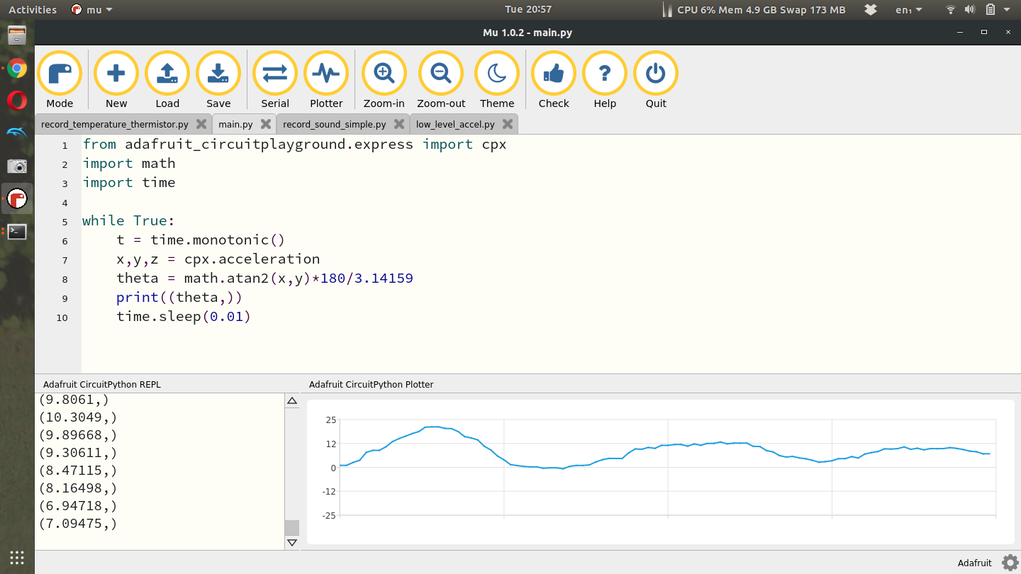
In this example I'm going to swing a pendulum in the X/Y plane of the accelerometer sensor so that I can ignore the Z axis data. I'm going to get the actual angle of the pendulum but if you're building something else you can ignore this part. You’ll notice that when you point the CPX directly at you with the cable pointing up the x axis reads around 0 and the y axis reads around gravity. If you then rotate the sensor so that the cable is coming out of the left side of the CPX, the x axis is reading about gravity while the y axis is zero. This means we can form a triangle and get the angle using these two axes using the equation below which gives angle in degrees.

$$\theta = tan^{-1}(x/y)\frac{180}{\pi}$$

On the CPX specifically we want to import the math module and use the atan2 function. When I swing the pendulum then this is the result I get from Plotter in Mu.

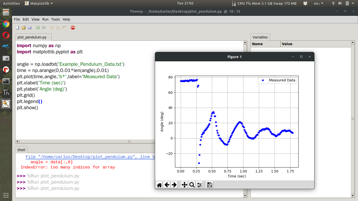
If I then bring this into Python I get the following plot below. In my data set I only logged the angle. Since the time step between each point was 0.01 seconds I was able to just create a time series. It’s pretty clear that there is some nonlinearity in the data so I chose to start the data at 0.5 seconds. Another thing I noticed was that the angle settled out to around 8 degrees so I chose to subtract off that bias from the angle data.

After trimming the data and removing some bias it was time to get my damping constant and damped natural frequency. There are a few equations that can help you obtain these parameters. First, the settling time is the length of time it takes for the oscillations to settle. The settling time can be used to find the damping constant. This is equal to:

$$\sigma = \frac{4}{T_s}$$

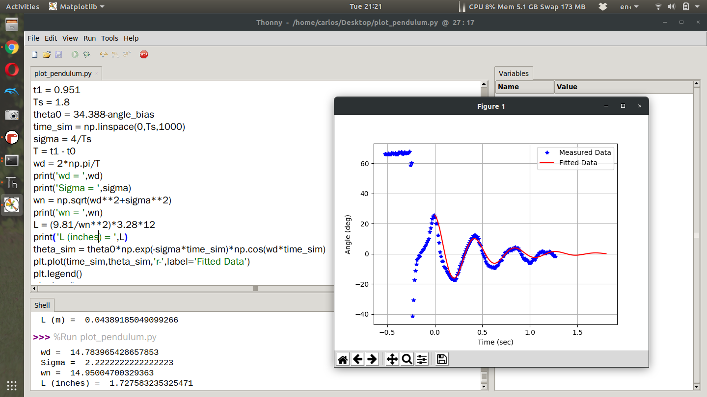
For my data set the settling time was about 1.25 seconds which gave a damping constant of 3.2. Once I had the damping constant I could obtain the damped natural frequency. This was done by measuring the distance between two peaks in the data set. There is a peak at around 0.5 seconds and another at around 0.95 seconds. I can use this to compute a period T. Period can be computed to angular frequency using the equation below.

$$\omega_d = \frac{2\pi}{T}$$

Using the period in my wave form I obtained a damped natural frequency of about 14.8 rad/s. Using these values I can plot the simulated data on top of the measured data noting that my initial angle was about 35 degrees minus the bias of 8 degrees. When I first plotted the data I noticed that my fit wasn’t entirely perfect. My period was correct but my damping rate was too high. I realized it was because my settling time was too big. I increased the settling time to 1.8 seconds and got this plot here. You can see that my fitted data lined up almost perfectly with my measured data.

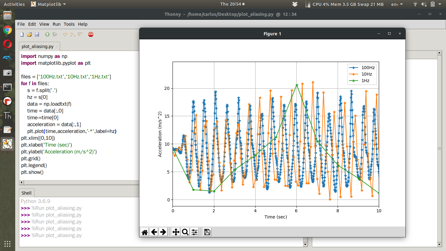
For the second part of this lab you need to vary the frequency somehow. In this case I changed the length of the pendulum which changed the natural frequency. I then proceeded to measure the angle as it oscillated at its natural frequency. I repeated this at sampling frequencies of 1, 10 and 100 Hz. The way I changed the sampling frequency was by changing the time.sleep value in the while True loop. The accelerometer code I used can be found on Github. After I finished the experiment I had 3 data files that I plotted on top of each other. This what I got with the longest string. It’s easy to see in the photo that sampling at 1 Hz was way too slow to capture the natural oscillations of the water bottle. However, 100 Hz and even 10 Hz was plenty fast to sample the oscillations. According to the recorded data there was above 19 cycles in 9 seconds which is about 2 Hz. In this case, as long as we sample at 4 Hz the signal will be captured properly which is why 10 Hz and 100 Hz is able to capture the signal correctly.

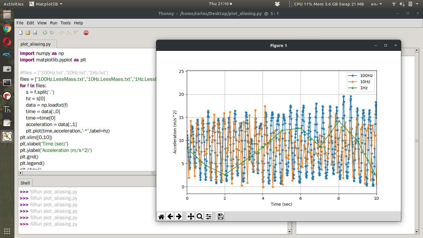
Once you sample your waveform at 3 different sampling rates I want you to change something about your setup. For example, you can drive slower or faster over the speedbump, you can change the length of your pendulum or the length of your ruler that you’re vibrating. I elected to shrink the length of the pendulum. This raised the natural frequency of the system by enough to change the results as shown in the figure below.

In this case you can see that there were 33 cycles in 10 seconds which is 3.3 Hz. The Nyquist criteria states that I need to sample at 6.6 Hz. The Nyquist criteria is very specific though in that if you sample at twice the frequency, you will just obtain the correct frequency. This does not mean that you will capture every data point properly. Hence in the chart above, the blue line at 100 Hz is perfect, the green line at 1 Hz is too slow (less than 6.6 Hz) and the orange line at 10 Hz captures the frequency correctly but between 5 and 8 seconds does not adequately capture the waveform.

Assignment

Upload a PDF with all of the photos and text below included. My recommendation is for you to create a Word document and insert all the photos and text into the document. Then export the Word document to a PDF. For videos I suggest uploading the videos to Google Drive, turn on link sharing and include a link in your PDF.

1. Include a video of you explaining your experiment. What state are you measuring? What is varying? Show the system varying and explain the code you are using the capture the data. Use the Plotter in Mu to show the system varying. (Make sure you introduce yourself in the video and that you show your face at some point) Explain what you changed about the system to change the natural frequency. I changed the length of my pendulum which changed the natural frequency. What did you change? - 20%

2. Take data at 3 different frequencies and two different configurations (a total of 6 data sets). Include two plots as I did above with appropriate labels and legends - 20%

3. Explain the results of your experiment in 1 or 2 paragraphs. Did you encounter any aliasing? Did the amount of aliasing change when you changed the parameters of your system? Why or why not? - 20%

4. Plot your measured data in Python for your lowest frequency and highest sampling rate and attach a well formatted figure. Include a plot of your fitted data alongside your measured data. Do they match? Why or why not? Write a paragraph explaining your result - 20%

5. Estimate your damping constant, damped natural frequency, damping ratio, and natural frequency. State these values explicitly in the submission Given the frequency you computed, comment on the frequency you would need to completely avoid aliasing and if the CPX is capable of doing that. - 20%